Stock Trading

Algorithm

June 2023

Select a version to view

Project Overview

This project implements a neural network-based stock trading system that learns optimal trading strategies through evolutionary learning. The system analyzes historical stock data (TSLA 1-minute candlesticks) and evolves a neural network to maximize a custom profit metric called the Profit Index.

                  Key Features:
                  Custom Neural Network: Built from scratch using NumPy
Evolutionary Learning: Weight optimization through iterative testing
Profit Index Metric: Custom performance evaluation function
Real-time Simulation: Backtest trading strategies on historical data
Visualization: Learning curves and equity performance graphs

               

Technology Stack

Python 3.x NumPy Matplotlib

Neural Network Architecture

Network Structure

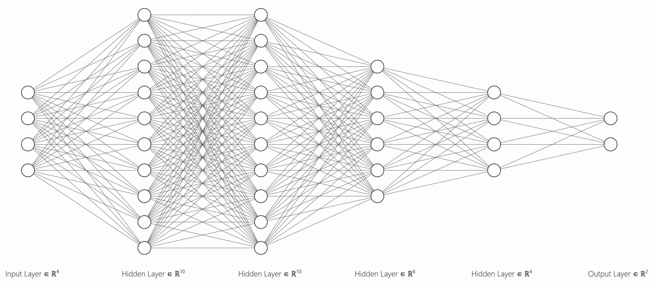
This is an exemplatory image of how a neural network looks like. Note that the layer size is depicted less complex for visualization purposes.

Layer Configuration: [40] → [100] → [100] → [60] → [20] → [2]

Input Layer → Hidden Layers (ReLU) → Output Layer (Softmax)

Layer	Type	Neurons	Activation	Purpose
Input	Dense	40	-	20 candles × 2 features (price + volume)
Hidden 1	Dense	100	ReLU	Feature extraction
Hidden 2	Dense	100	ReLU	Pattern recognition
Hidden 3	Dense	60	ReLU	Feature reduction
Hidden 4	Dense	20	ReLU	Decision preparation
Output	Dense	2	Softmax	Buy/Sell probabilities

Input Features

The network processes 20 consecutive 1-minute candles with the following features:

Open Price: Opening price of each candle
Volume: Trading volume for each candle
Moving Average: 20-period simple moving average

Total Input Size: 40 features (20 candles × 2 features per candle) + moving average

Output Layer

The network outputs two probability values:

Buy Signal [0]: Confidence in upward price movement
Sell Signal [1]: Confidence in downward price movement

Learning Algorithm

Profit Index Calculation

The system uses a custom metric called the Profit Index to evaluate neural network performance:

Profit_Index = Σ (max(prediction) - 0.5) × direction × actual_price_change / n_datasets

Python

class ProfitIndex:
            def forward(self, y_pred, price_changes):
                sum = 0
                for i, dataset in enumerate(y_pred):
                    y_pred_clipped = np.clip(dataset, 1e-7, 1-1e-7)
                    
                    # Extract confidence (0 to 0.5 range)
                    max_confidence = np.max(y_pred_clipped, axis=1) - 0.5
                    
                    # Determine direction: +1 for buy, -1 for sell
                    direction = (np.argmax(y_pred_clipped, axis=1) * (-2)) + 1
                    
                    # Calculate weighted profit
                    sum += np.dot(max_confidence, direction) * price_changes[i]
                    
                return sum / n_datasets_per_gen

Weight Optimization Strategy

1. Initialization

Python

self.weights = 0.1 * np.random.randn(n_inputs, n_neurons)
        self.biases = np.zeros((1, n_neurons))

2. Iterative Modification

The system uses two modification strategies:

Full Weight Modification (90% of iterations):
                  Python
def modify_weights():
            for layer in layers:
                layer.type.weights += variation_factor * np.random.randn(n_inputs, n_neurons)
                layer.type.biases += variation_factor * np.random.randn(1, n_neurons)

Partial Weight Modification (10% of iterations):
                  Python
def modify_partial_weights():
            for layer in layers:
                rw = randrange(len(layer.type.weights))
                rb = randrange(len(layer.type.biases))
                layer.type.weights[rw-1] += variation_factor * np.random.randn(layer.type.n_neurons)
                layer.type.biases[0][rb-1] += variation_factor * np.random.randn(1)

3. Selection Process

Python

for iteration in range(n_generations):
            # Modify weights
            if iteration % 10 == 0:
                modify_partial_weights()
            else:
                modify_weights()
            
            # Test new configuration
            load_data()
            output = process_inputs()
            pi = ProfitIndex().forward(output, Y)
            
            # Keep if better, revert if worse
            if pi > best_profit_index:
                saveWeightsBiases()
                best_profit_index = pi
            else:
                loadBestWeightsBiases()

Activation Functions

ReLU (Hidden Layers)

f(x) = max(0, x)

Python

class Activation_ReLU:
            def forward(self, inputs):
                self.output = np.maximum(0, inputs)

Custom Softmax (Output Layer)

Modified softmax with decision bias parameter:

Python

class Activation_Softmax:
            def forward(self, inputs):
                # Normalize with decision bias
                values = inputs / ((abs(np.max(inputs, axis=1, keepdims=True)) + 
                                abs(np.min(inputs, axis=1, keepdims=True)) * decision_bias))
                
                # Apply exponential normalization
                self.output = np.exp(values) / (np.max(np.exp(values)) + 
                                                np.min(np.exp(values)))

How This Model Learns

The learning process works through trial and error:

Start with a random guess - The model begins with random weights (like a student guessing without knowledge)
Make predictions - It analyzes 200 random time windows from the stock data and predicts whether prices will go up or down
Score the performance - A "Profit Index" measures how good those predictions were (like grading a test)
Randomly tweak the understanding - The model makes small random adjustments to its weights and biases (like the student trying a slightly different approach)
Keep improvements, discard failures - If the new predictions score better, keep the changes. If worse, revert back to the previous version
Repeat 300 times - This cycle runs 300 generations, gradually finding better and better configurations

Decision Bias (0.15): Controls the differentiation strength between buy and sell signals.

Lower bias (0.05): More extreme decisions (72% buy vs 28% sell)
Higher bias (0.15): More balanced decisions (58% buy vs 42% sell)

Implementation Details

Configuration Parameters

Parameter	Value	Description
`n_neurons`	[100, 100, 60, 20]	Hidden layer neuron counts
`n_candles`	20	Candlesticks per input window
`variation_factor`	0.001	Weight modification magnitude
`n_datasets_per_gen`	200	Training samples per generation
`n_generations`	300	Total optimization iterations
`decision_bias`	0.15	Buy/sell differentiation strength

Data Loading Process

Python

def load_data():
            with open('TSLA_1min_sample.txt') as input_file:
                X.clear()
                Y.clear()
                line_ranges = []
                
                # Generate random time windows
                for iteration in range(n_datasets_per_gen):
                    i = np.random.randint(dataset_line_number - n_candles)
                    line_ranges.append([i, i + n_candles - 1])
                    X.append([])
                    moving_average.append(0)
                
                # Parse candlestick data
                for i, line in enumerate(input_file):
                    for num_dataset in range(n_datasets_per_gen):
                        if i >= line_ranges[num_dataset][0] and i <= line_ranges[num_dataset][1]:
                            datetime_input, data_open, high, low, close, volume = (
                                item.strip() for item in line.split(',', 5))
                            
                            X[num_dataset].append(float(data_open))
                            X[num_dataset].append(float(volume))
                            moving_average[num_dataset] += float(data_open)
                        
                        if i == line_ranges[num_dataset][1]:
                            # Calculate target (price change percentage)
                            Y.append(((float(close) - float(data_open)) / 
                                    float(data_open)) * 100)
                            
                            # Add moving average feature
                            moving_average[num_dataset] *= (1 / n_candles)
                            X[num_dataset].append(moving_average[num_dataset])

Forward Propagation

Python

def process_inputs():
            outputs = []
            for dataset in X:
                # First layer
                layers[0].type.forward(dataset)
                layers[0].function.forward(layers[0].type.output)
                
                # Remaining layers
                for i, layer in enumerate(layers[1:]):
                    layer.forwardType(layers[i].function.output)
                    layer.forwardFunction(layer.type.output)
                
                outputs.append(layers[-1].function.output)
            return outputs

Trading Simulation

After training, the system runs a realistic trading simulation to evaluate actual performance.

Simulation Parameters

Starting Capital: $1,000
Position Sizing: Dynamic based on signal confidence
Test Period: ~8,248 minutes of historical data
Asset: Tesla (TSLA) stock

Position Management

The system dynamically adjusts position sizes based on prediction confidence:

Position_Size = (Confidence - 0.5) × 2 × Total_Equity

Python

def execute_trade(response, currentPrice, equity):
            if response[0][0] > response[0][1]:  # Buy signal
                confidence = response[0][0]
                position_size = (confidence - 0.5) * 2 * equity
                shares = position_size / currentPrice
                
                print(f"Buy {shares:.2f} shares worth ${position_size:.2f}")
                
            else:  # Sell signal
                confidence = response[0][1]
                position_size = -(confidence - 0.5) * 2 * equity
                shares = position_size / currentPrice
                
                print(f"Sell {-shares:.2f} shares worth ${abs(position_size):.2f}")

Performance Metrics

The simulation tracks multiple performance indicators:

Total Equity: Cash + Position Value
Percentage Return: (Final Equity / Initial Capital) - 1
Outperformance: Strategy Return / Buy-and-Hold Return
Profit Index: Risk-adjusted performance metric

Training Process

During training, you'll see output like:

Python

---------------START DEEP LEARNING----------------

        LAYER FIRST
        LAYER NR 0
        LAYER NR 1
        LAYER NR 2
        LAYER NR LAST
        Iteration 0 done, ProfitIndex: 0.0123

        Better Configuration found in Iteration 15, ProfitIndex: 0.0187
        Better Configuration found in Iteration 42, ProfitIndex: 0.0234
        Iterations 10% completed
        Better Configuration found in Iteration 89, ProfitIndex: 0.0301
        Iterations 20% completed
        ...
        Iterations 100% completed

        All iterations done! Time passed: 245 seconds

Simulation Output

Python

---------------START TRADING SIMULATION----------------

        Line ranges: [1523, 9771]
        Bought 45.32 Shares worth $982.50
        Sold 12.15 Shares worth $265.80. Profit: $18.45
        ...
        ENDING EQUITY: 1156.78
        ENDING OUTPERFORM: 1.23

Interpretation:

Final equity of $1,156.78 represents a 15.68% return
Outperformance of 1.23 means the strategy beat buy-and-hold by 23%
This signals strong model performance at first glance

Disclaimer: However, after thorough analysis, these results were not representative of the models true capabilities. The next section will demonstrate why.

Performance Analysis

Visualization

To analyze, whether the results were truly as promising as they seemed the following comprehensive performance visualizations were generated:

                  Trading Performance Graph
                  Blue Line: Strategy equity percentage change
Red Line: Stock price percentage change
Green Line: Outperformance ratio

               

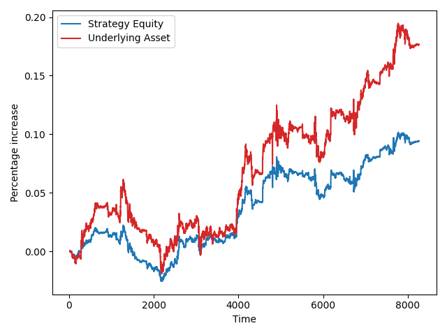
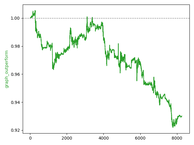
Immediately, it is obvious that instead of scalping the markets, the bots success was due to the great performance of the underlying asset. In long term, the strategy severely underperforms the buy-and-hold strategy even when simulated multiple times.

                  Learning Curve Graph
                  Green Line: Best Profit Index over generations
Red Line: Test Profit Index per iteration

               

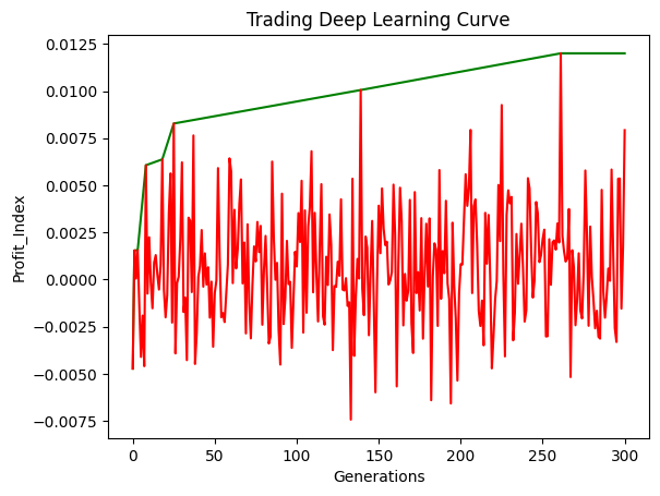
This hypothesis is further supported by the learning curve graph, which shows that the model does not seem to learn meaningful relationships. Instead, it randomly finds profitable strategies that most likely resemble unprecise forms of the "buy-and-hold" strategy. Due to fluctuations in confidence, the model randomly fails to hold or even sells the asset and misses out on equity gains, underperforming "buy-and-hold".

Due to limited available free market data the outcome of this project was never to create a perfectly working model. This is why i stopped development at this point, as in my opinion the model coming up with a profitable strategy (even if it is a worse verison of buy-and-hold) is a (small) success. Preventing the model from falling into this 'local minimum' would take lots of time and ML experience which I did not have at that point in time.

Learnings

Key Takeaways:

Due to significant underperformance and clear learning issues, the model is not viable for practical use
However, this project provided me with valueable, deep insights and enhanced my understanding of machine learning and the technical foundations behind popular libraries like TensorFlow or PyTorch.

Since the completion of this project, more than 2 years have passed. In the meantime, my knowledge and skills in machine learning have significantly advanced. If i were to continue this project today there is a lot of things, i would do differently. Some of them iclude:

               Opportunities for future enhancement
               Switching to a library like TensorFlow would simplify model development and give opportunity to focus on improving model significance and performance
More technical input features like indicators (RSI, MACD, price momentum) could be incorporated
Proper training and validation splits to avoid overfitting and data leakage
Use a recurrent network (instead of Dense Layers) to capture temporal dependencies in the time-series stock price data
Use gradient-based optimization for more efficient training
Normalize input features (volume has a different scale than stock price)
Detrend the market data or use more data from more diverse market conditions

            

Neural Network Stock Trading System

A learning-focused machine learning project built entirely from scratch — demonstrating my ability to design, optimize, and evaluate neural networks without relying on pre-built ML frameworks.

Project Overview

This project is a self-built neural network trading system that analyzes minute‑level stock data and attempts to generate buy/sell decisions. The focus of this project was not to build a profitable trading bot, but to fully understand how neural networks work at the lowest level — from matrix operations to training logic.

            Why this project matters:
            I implemented a complete neural network using only NumPy — no TensorFlow, PyTorch, or ML libraries.
I created a custom learning and evaluation strategy to optimize the model.
I simulated trading decisions and evaluated them with a performance metric I designed myself.
The project shows my ability to work independently, build complex systems, and quickly learn advanced ML concepts.

         

How the System Works

The model takes short windows of historical TSLA price data and outputs a probability for buying or selling. Instead of classical backpropagation, I used a simple evolutionary strategy, repeatedly adjusting the model’s weights and keeping the best-performing version.

Key Components

Custom Neural Network: Several fully connected layers coded manually.
Evolutionary Training: Small informed changes to the model, keeping better-performing generations.
Profit Index: My own scoring function to judge trading performance.

Simulation & Testing

I ran the model across historical 1‑minute TSLA data, simulating buy/sell decisions. The Profit Index rewarded:

Correct direction predictions
High-confidence decisions
Stable, repeatable performance over many data slices

The simulation results were not profitable — but they revealed how tiny weight changes influenced model behavior, and gave me hands‑on intuition about training dynamics.

Results

While the system did not produce a profitable trading strategy, it successfully demonstrated that:

I can independently design and implement a multi-layer neural network.
I understand how data preprocessing, weight initialization, activation functions, and output interpretation work under the hood.
I can build custom evaluation metrics and training loops without relying on existing tools.

What I Learned

This project provided deep, practical intuition about modern machine learning. Key learnings include:

How neural networks behave internally (beyond high-level libraries)
How to structurally debug ML models and interpret unstable learning behavior
The challenges of financial time‑series prediction
How to design experiments, evaluate performance, and iterate methodically

            In short: This project wasn’t about creating the perfect trading bot — it was about building ML fundamentals from the ground up. It showcases my ability to tackle complex problems independently, understand the math behind machine learning, and apply these skills in practical scenarios.
         

Neural Network Stock Trading System

A learning-focused machine learning project built entirely from scratch — demonstrating my ability to design, optimize, and evaluate neural networks without relying on pre-built ML frameworks.

Project Overview

                Why this project matters:
                I implemented a complete neural network using only NumPy — no TensorFlow, PyTorch, or ML libraries.
I created a custom learning and evaluation strategy to optimize the model.
I simulated trading decisions and evaluated them with a performance metric I designed myself.
The project shows my ability to work independently, build complex systems, and quickly learn advanced ML concepts.

            

How the System Works

Key Components

Custom Neural Network: Several fully connected layers coded manually.
Evolutionary Training: Small informed changes to the model, keeping better-performing generations.
Profit Index: My own scoring function to judge trading performance.

Architecture

Illustration of the multi-layer network used (simplified for visualization).

Simulation & Testing

I ran the model across historical 1‑minute TSLA data, simulating buy/sell decisions. The Profit Index rewarded:

Correct direction predictions
High-confidence decisions
Stable, repeatable performance over many data slices

The simulation results were not profitable — but they revealed how tiny weight changes influenced model behavior, and gave me hands‑on intuition about training dynamics.

Results

While the system did not produce a profitable trading strategy, it successfully demonstrated that:

I can independently design and implement a multi-layer neural network.
I understand how data preprocessing, weight initialization, activation functions, and output interpretation work under the hood.
I can build custom evaluation metrics and training loops without relying on existing tools.

What I Learned

This project provided deep, practical intuition about modern machine learning. Key learnings include:

How neural networks behave internally (beyond high-level libraries)
How to structurally debug ML models and interpret unstable learning behavior
The challenges of financial time‑series prediction
How to design experiments, evaluate performance, and iterate methodically

                In short: This project wasn’t about creating the perfect trading bot — it was about building ML fundamentals from the ground up. It showcases my ability to tackle complex problems independently, understand the math behind machine learning, and apply these skills in practical scenarios.
            

Overview

This project explores how machine learning (ML) can be used to predict short-term stock price movements.

Inspired by a YouTube video on algorithmic trading, I decided to rebuild and improve a similar model from scratch in Python to better understand the fundamentals of Neural Networks.
The goal was not to create a profitable trading algorithm, but to learn the underlying mechanics of predictive financial modeling and backtesting.

How it works

1

Market Data

Tesla 1-min Price Data gets loaded

2

Neural Network

A neural network is trained to predict whether the next candle will be bullish or bearish

3

Trained Model

The model predicts a numeric value from -1 (100% SELL) to 1 (100% BUY) for the next candle

4

Backtesting

The model and its returns are tested in a trading simulation also made in python

Stock Trading

Algorithm

Select a version to view

Project Overview

Key Features:

Technology Stack

Neural Network Architecture

Network Structure

Layer Configuration: [40] → [100] → [100] → [60] → [20] → [2]

Input Features

Output Layer

Learning Algorithm

Profit Index Calculation

Weight Optimization Strategy

1. Initialization

2. Iterative Modification

3. Selection Process

Activation Functions

ReLU (Hidden Layers)

Custom Softmax (Output Layer)

How This Model Learns

Implementation Details

Configuration Parameters

Data Loading Process

Forward Propagation

Trading Simulation

Simulation Parameters

Position Management

Performance Metrics

Training Process

Simulation Output

Performance Analysis

Visualization

Trading Performance Graph

Learning Curve Graph

Learnings

Key Takeaways:

Opportunities for future enhancement

Neural Network Stock Trading System

Project Overview

Why this project matters:

How the System Works

Key Components

Simulation & Testing

Results

What I Learned

Neural Network Stock Trading System

Project Overview

Why this project matters:

How the System Works

Key Components

Architecture

Simulation & Testing

Results

What I Learned

Overview

How it works

1

Market Data

2

Neural Network

3

Trained Model

4

Backtesting

Step 1

Loading Market Data

1-Minute TESLA stock data was downloaded from Yahoo Finance